Delineate snow using Normalized Difference Snow Index, Sentinel 2 and QGIS

The Sentinel-2 mission is a land monitoring constellation of two satellites that provide high resolution optical imagery and provide continuity for the current SPOT and Landsat missions.

Sentinel-2 satellite data is provided in multiple levels and stages of processing, from raw data to already TOA, geometric and radiometric calibration (Level-0, Level-1A, Level-1B and Level-1C).

SENTINEL-2 products available for users are:

Making a difference between clouds and snow using optical imagery can be difficult. Clouds are always a problem in optical imagery, affecting and altering all the information from a scene. In this example we will investigate which level of Sentinel-2 images are optimal for our studies, how to download them and how to make the difference between the clouds and snow pixels, using band operations and the Normalized Difference Snow Index.

Best choice when it comes to Sentinel-2 data are Level-1C products which are radiometric and geometric corrected TOA products. No prior preprocessing is required.

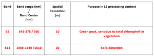
In order to detect the snow in the electromagnetic spectrum, we will use the information included in the range of 0.66 and 1.6mm due to the reflective propriety of snow at 0.66 mm and not reflective propriety at 1.6mm.

Sentinel-2 bands that acquire information in these two ranges of the electromagnetic spectrum are Band 3 and Band 11.

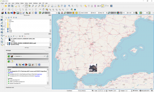
Step 1: Download Sentinel 2 data using Semi-Automatic Classification Plugin available with QGIS. Let’s see how we can make the difference between these two (clouds and snow) using QGIS (an open source, easy to handle GIS software product). For these exercise we will use an Sentinel-2 image from the area of Sierra Nevada mountains. Permanent snow can be found on the top of these mountains.

1.1 Open QGIS, open Semi-Automatic Classification Plugin (install it if you do not have it).

1.2 Press the Download images tab, insert your Copernicus Open Access Hub credentials (go to https://scihub.copernicus.eu/dhus/ and create an account if you do not have an account)

1.3 Use the location button in order to define a region of interest, insert the desired dates for image acquisition and click Find (see the red squares in the image below).

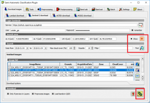
1.4 Select the desired image from the list and then click the Run button.

1.5 This operation will download in your computer the bands of the Sentinel 2 image you selected separately.

IMPORTANT!! All downloaded bands have different spatial resolution.

Step 2: Calculate the Normalized Difference Snow Index

2.1 For this calculation we need to use Band 3 and Band 11. We can observe that the spatial resolution of these two is different. In order to perform operation with the bands we need to resample the raster’s to the same spatial resolution

2.2 Band 3 already has a spatial resolution of 10 m. We need to resample only Band 11. Right click on Band 11 > Save as > in the Resolution Tab introduce 10 m. In order to avoid errors, perform the same operation for Band 3 also.

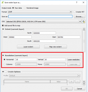
2.3 Go to Raster > Raster calculator and introduce the NDSI formula (B3-B11)/(B3+B11).

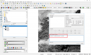
2.4 The NDSI will be displayed

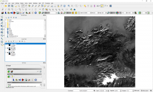
2.5 Explore the raster histogram Right click on the raster in Layer Panel and select Proprieties

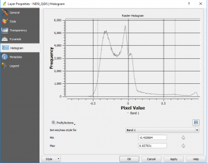
2.6 The pixel values are between -1 and 1, we can consider that the calculations were done in a correct way.

• pixels with strong NDSI negative values are considered as cloud-free.
• most potential cloudy pixels have NDSI values in a range between -0.1 and +0.2.
• pixels that have NDSI value under 0.20, they are considered as ‘no snow’ pixels.
• pixels with high NDSI as ‘snow’ pixels are considered snow pixels. Different thresholds are required for better snow delineation.

Step 3 Let s check if the statements above are true.

3.1 In order to do this we will create a mask for delignating the range of pixel values that interest us.

3.2 Mask snowy pixels (range above 0.8). Go to Raster Calculator and enter the next formula “NDSI_QGIS@1″ > 0.8. This will create a mask that will delineate only high potentially snow pixels.

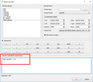
3.3 The mask pixel values will have two values 0 or 1. Your result will probably look like this.

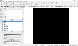
3.4 In order to delineate the snow pixels go to Proprieties and in the color gradient replace 0 with 1.

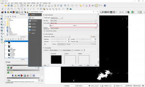
3.5 This will show the high potential snow pixels.

3.6 We can convert the Raster to Vector for a better visualization using the same QGIS function. Go to Raster > Conversion > Raster to Vector.

3.7 Symbolize the new layer

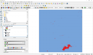
3.8 Verify the results

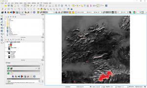
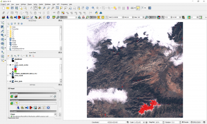
3.9 The area that match with Sierra Nevada Mountain is the one covered in snow. Red area in the images above.

Step 4. Repeat the methodology used at step 3 in order to delineate cloud related pixels. Use pixels range values between -0.1 and +0.2.

Quality training taught by professionals

RECOMMENDED COURSES